
Multi-class Classification of Tweets
Introduction & Data
This project aims to do a multi-class classification on tweets. The “success” of any of the methods we have run, is based on the cost returned to us by the leaderboard. The data provided was as follows:
- train.mat : This contained X train bag, Y train and train raw. As the name suggests, X train bag was the training data set. This was a sparse matrix, which had under each feature(columns), the number of times each word from the vocabulary set had been seen in the respective tweet (rows). train raw had the raw tweets.
- validation.mat : This contained X validation bag, and validation raw. These data sets are to validate our classification.
- vocabulary.mat : This contained just a single row matrix of strings containing all possible words in the vocabulary of the data set.
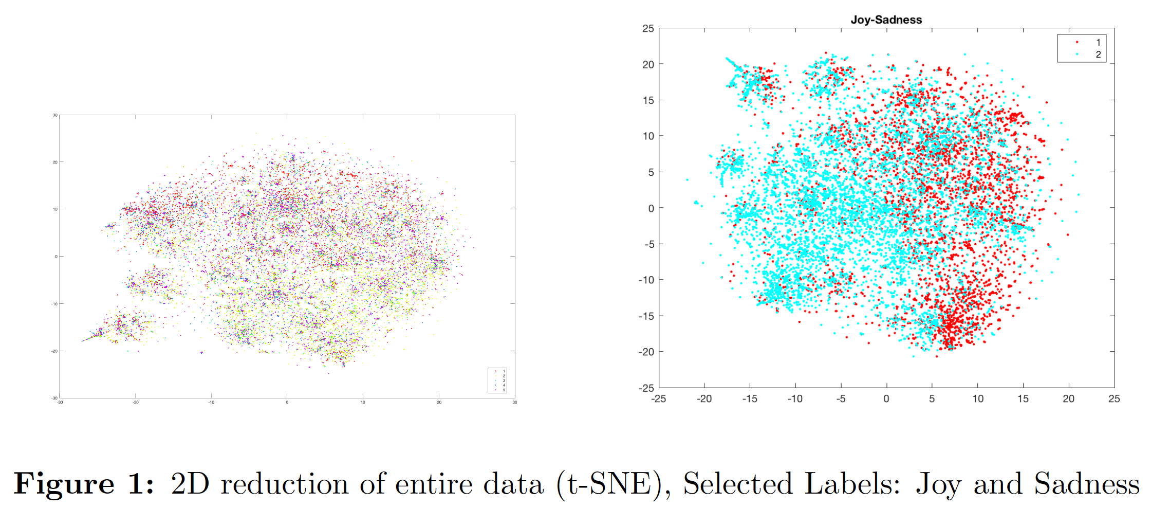
The figure on the left is the 2D representation of the entire dataset using the t-SNE algorithm. No clear patterns were observed so another plot of only contrasting labels (Joy and Sadness) was created as shown on the right. There is a visible division between the joy labels(red) and sadness labels(blue) that could be classified fairly well using a linear decision boundary. This was the first clue that models generating linear decision boundaries can work well with this dataset.
Initial Methods - Baseline 1
For this baseline, it was our first attempt to just run a variety of models on the data, without any pre-processing. The methods we tried were as follows:
-
Logistic Regression We used liblinear package to train the model using multi-class logistic regression. We obtain the probabilities of each observation belonging to class 1 through 5. Here, we used the asymmetric cost matrix multiplied with the obtained probabilities. This gives us the cost of misclassification given a prediction. We chose the label with minimum cost as the prediction.
-
Naive Bayes We used the ‘ fitcnb’ function in MATLAB with a multinomial distribution to train our model parameters using the given training bag-of-words. This gave us a validation cost of 0.9447. Since Naive Bayes works well for most text classification purposes, this was our first attempt. Although the obtained cost is pretty decent for a basic model like Naive Bayes, it wasn’t the best performing model because of the conditional independence assumption it makes on the features.Since we dealt with a bag of words model, Naive Bayes assumed each word to be independent of the other in a tweet. This is not a great assumption since it misses out on capturing context. An improvement to Naive Bayes could have been achieved by generating bi-grams instead of the currently used uni-grams. Although we did generate bi-grams(See Appendix) from the raw texts to test this hypothesis, the number of features exploded to 134,000 from the current 10,00 and it became too large to model in the specified time. We would like to develop a feature selection routine for the bi-gram model to test the algorithm’s performance in the future.
-
SVM We used the ‘svmtrain’ function from MATLAB’s libsvm package to train our SVM models. The ‘svmpredict’ function was used to generate probabilities for each label for each tweet. These probabilities were multiplied with the cost matrix to generate mean loss for each label. The label with the lowest mean loss was selected as the final prediction for an input tweet. We trained SVM models with both polynomial and rbf kernels. Cross validation was performed to tune the degree and cost parameters for the polynomial kernel and kernel width and cost parameters for the rbf kernel.
Continuing Methods - Baseline 2 and onwards
Pre-processing the bag of words
After successfully crossing Baseline 1, we started trying many different preprocessing approaches to reduce the number of dimensions and normalize the data in order to get to a lower cost. They are as follows:
- Feature Selection:
- Grouping Words which mean the same thing: For this, we grouped features which meant the exact same word, since we assumed they would imply the same sentiment. For example, we grouped “tomorrow” and “2morrow”
- Grouping singular and plural of the same word: For this, we grouped the singular and plural of nouns such as “text and “texts”
- Grouping smileys: Here, smiley icons which meant the same thing were grouped - such as “:)” and “=]”
-
Removing Numbers: We assumed that numerical values wouldn’t add or take much from the sentiment of a tweet, and for this reason we experimented with removing all number-features. There were about 240 such features.
-
Removing “<user>“: All usernames were represented as <user>. We removed these features as they do not add to the sentiment of the sentence.
- Term Frequency-Inverse Document Frequency (TF-IDF): TF-IDF pre-processes to
data to remove bias on sentence length and by giving lesser weight to stopwords. We tried two
variations of TF-IDF and achieved significantly different results. As a step prior to TF-IDF,
we normalized each word count by dividing it by total number of words in a given tweet.
These are mentioned below:
- $ tfidf(T,D) = f_{t,D}log(abc/dF) $
(y_0 + a^2)